# View Measurements

Measurements saved in the applications Notebook can be viewed alone or multiple together (The Notebook). The data can also be exported to be used in other applications.

# Traces

# Show/Hide Traces

Individual traces can be hidden by clicking on their corresponding rows in the table. Hidden traces are indicated by a greyed out text color in the table. Another click on the table row will will show the hidden trace again.

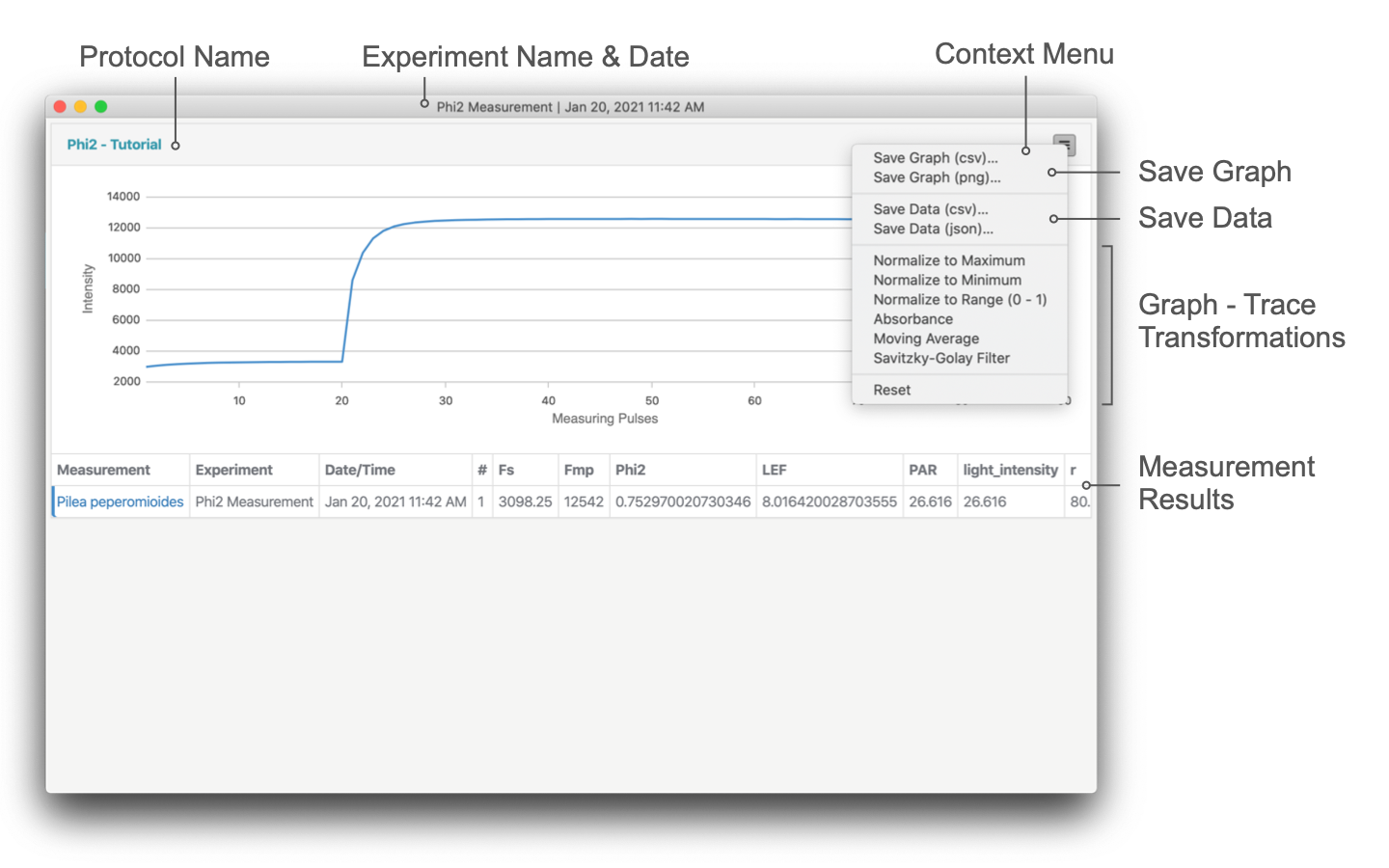
# Export Traces

The traces currently viewed can be exported either as a .png image or a .csv file. Click on the menu button ☰ in the right corner of the panel header and select Save Graph (png) or Save Graph (csv) from the context menu and select a filename and location to save. Always the current traces are saved, so when transformations were applied, those changes are saved.

# Transform

The traces displayed in the graph can be transformed using the available methods listed in the table below. These are very basic implementations intended to provide tools to quickly apply and compare results. If more sophisticated transformations are needed or for example, the normalization is supposed to be at a certain position in the trace and not the max/min, it would need to be implemented in a macro.

The transformations work accumulative, so first the Absorbance could be calculated and afterwards the resulting absorbance traces could be normalized or smoothed.

All changes can be un-done, selecting Reset from the context menu. The results are always temporary and are not saved with the measurements.

Transformation	Details
Normalize to Maximum	Normalize all values to the maximum value of a trace $x'={\frac{x}{\text{max}(x)}}$
Normalize to Minimum	Normalize all values to the minimum value of a trace $x'={\frac{x}{\text{min}(x)}}$
Normalize to Range (0 - 1)	Normalize to the range between 0 - 1 $x'={\frac{x-{\text{min}(x)}}{\text{max}(x)-\text{min}(x)}}$
Absorbance	Calculating the absorbance using the first value of the trace as $I_{0}$ $A={-\log_{10}\left(\frac{I}{I_{0}}\right)}$
Moving Average	Apply a simple moving average to smooth trace (n=3) $\overline{y}_{t}={\frac{y_{t} + y_{t-1} + y_{t+1}}{n}}$
Savitzky-Goley Filter	Simple smoothing filter based on Savitzky-Goley $\overline{y}_{t}={\frac{(-2 * y_{t-3} + 3 * y_{t-2} + 6 * y_{t-1} + 7 * y_{t} + 6 * y_{t+1} + 3 * y_{t+2} + -2 * y_{t+3})}{21}}$

# Table

Most of the data that is calculated based on traces or kinetics measured with the MultispeQ's IR and visible detectors. These derived values are displayed in the table underneath the section for graphing these traces. These can be numeric, but also categorical values. In the case the original recorded trace needed to be transformed to derive parameters, they can be returned and displayed as inline graphs within the table.

# Inline Traces

With more complex Protocols using the _protocol_set_ command, probably more than one trace is being recorded and it can be helpful to view and compare kinetics side by side. To view and explore the traces, click on one of the traces in the table column of interest to load all traces into the graph view.

Inline Graph Limitations

Due to the small size of the graphs within the table the maximum number of data-points is limited to 10,000. In case the traces exceed this length, only the first 10,000 data-points are displayed and the color is changed to red instead of the usual blue to indicate a longer trace. When selected to be displayed, the full length trace is shown.

# Export Data (csv)

The data from the measurement results can be exported as a csv file. Simply click on the menu button ☰ in the right corner of the panel header and select Save Data (csv) from the context menu and save the file to a selected location. When different Protocols were used in one Measurement or Measurements with different Protocols are selected at the same time, the data will only be saved for the corresponding panel.

Since some columns might hold traces, that are comma separated themselves, the traces are saved as strings, meaning they are enclosed in double quotes (e.g. "1,2,5,3,..."). So when importing the data into a program like Excel, make sure to set the delimiter to comma , and the Text qualifier to ". In a second step, the column with the traces, can be properly imported using the Text to Columns feature.

# Export Data (JSON)

The data from measurement results can be exported as a json file as well. The data has the same structure as a csv and might be easier to import/parse when having a lot of traces in the measurement results. Simply click on the menu button ☰ in the right corner of the panel header and select Save Data (json) from the context menu and save the file to a selected location. When different Protocols were used in one Measurement or Measurements with different Protocols are selected at the same time, the data will only be saved for the corresponding panel.

Data Compatibility (JSON)

In case you work with the software package for R or Jupyter, you can only use it with PhotosynQ Projects at this point.

← The Notebook Protocols →